Support vector machine - Linear
The Support Vector Machine
Support vector machine is a classification algorithm. The idea behind the algorithm is that it tries to seperate 2 different labeled datasets. Compared to kNN and RandomForest, this is a supervised algorithm. Hence meaning that we use our labeled data to divide/classify our datapoints.
We divide the dataset utilizing a hyperplane. A hyperplane is a function of degree (Features-1), 2 features will entail a function of degree 1 (a line). 3 features will be a 2 dimensional plane. 4 features will be a 3 dimensional function, eg. a box that encompases 0-labeled features and the 1-labeled features are outside the box.
Not only do we want to seperate the datapoints into their assiciated labels, we also want to maximize the distance that our datapoints has to the hyperplane (the border). Reasoning for this is that we want to avoid future datapoints (test set) slipping over the hyperplane because the hyperplane was just barely seperating some part of our dataset (confidence).
The SVM algorithm utilizes what is called a margin. The margin is what gives us a buffer between the two sets. In our case we have two labels so we will try to divide our set into two.
Support vectors are used to change the margin. We choose the datapoints that are closest to the hyperplane, this could be x number of points or the closest in distance with some variance. Only looking at the points that are closest to the margin will only work in the case that we have a purely seperable set. Incase that some datapoints lie in the other camp, we will have to take a look at all of the datapoints.
Our optimization of the margin will thus have to reflect, how many points we can afford to misclassify while keeping the maximum margin.
Svm with C = 10
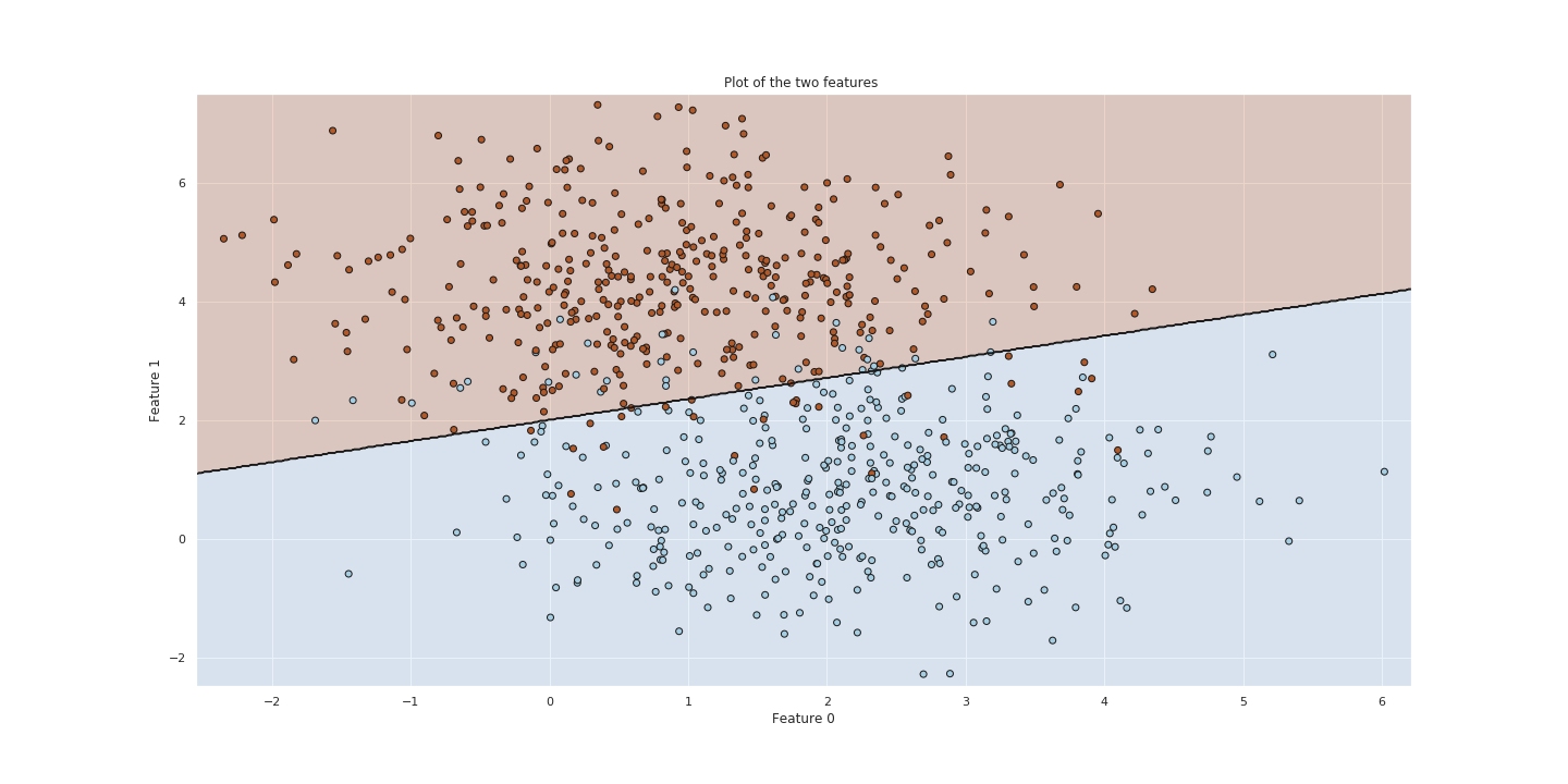
Let us try to use the SVM function from sklearn and then optimize the parameters to fit our dataset. We fit the model to our training set with a C = 10. The C parameter indicates to the SVM optimization how much we weight misclassifications.
Large C, the optimization will prioritize a smaller-margin hyperplane.
Other the other hand, a small value of C will cause the optimizer to prioritize larger-margin separating hyperplane, even if that hyperplane misclassifies more points.
Choosing a value of C = 10 is relatively high.
Optimizing The Model
We will now try to find the optimal C, that classifies our datapoints with the highest accuracy.
We do this by evaluating the model for different values of C. The C values we choose are
[0.00001, 0.001, 0.01, 0.1, 1, 10, 100] .
We can later run the evalutaion again if we find out that the C value is much higher for eg. 100. Then we might try to evaluate the model for values around this parameter.
When we evaluate the model we get the following accuracies corresponding to the C- parameters
{1e-05: 0.46875, 0.001: 0.925, 0.01: 0.925, 0.1: 0.93125, 1: 0.925, 10: 0.925, 100: 0.925}
We see that the value for C=0.1 has a bit of a higher accuracy than the values around it. We could try to narrow the range of the C parameter down even more, but we do not expect it to increase in accuracy that much.
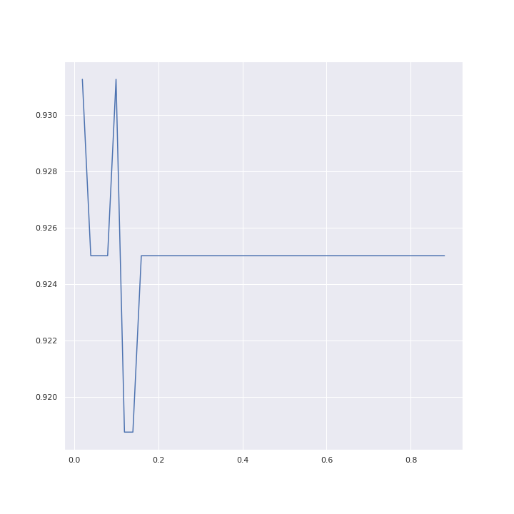
But lets try for value ranging 0.02 to 0.9.
narrowParameterList = np.arange(0.02, 0.9, 0.02).tolist()
print(narrowParameterList)
narrowTester = CrossValidation_SVM(n_folds = n_folds, parameterCList = narrowParameterList)

narrowClf , narrowAccuracyList = narrowTester.getOptimalSMV(x_train,y_train)
print(narrowClf)
In the figure below we can see that we get the same accuracy whether we are using C=0.02 or C=0.1
Testing model on test set
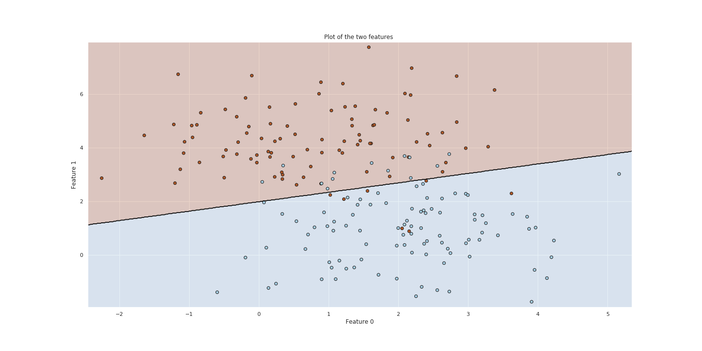
Now that we have a model with an optimal parameter for C, lets try to use it to predict on our test set.
In the figure below we can see the plot for our test set and the hyperplane that separates them. We see that there are quite a few blue data points on the red side of the border. This is in constrast to our train set which had near the same amount of blue and red points on the opposite of the side that they belong to.
To conclude
Optimizing the SVM on parameter C we get an accuracy of 0.925% which is fairly good considering that we have a nonseperable dataset using a linear seperator.
Further exploration
We in this case had a fairly simply case with only two features and they were somewhat separable by a 1 degree hyperplane (linear line). We could place the hyperplane quite easily.
If we had an example with 0-labeled datapoints surrounded by a donut or circle of 1-labeled datapoints, it would be quite difficult two utilize the linear kernel. A kernel of a different kind could be used to project data into another feature space.