PCA and classifications
Principal component analysis:
Some few tool to analyze the specific impact of each feature, and their impact on the label.
The tool is applied to a dataset of flowers, where we try to classify which features of the plant correspond to the specific flower.
We have four features sepal width, sepal length, petal width, and petal length. All are in cm.
The labels or the flowers we are trying to classify are Iris Setosa (label = 0), Iris Versicolour (label = 1), Iris Virginica (label = 2)
PCA
We only have 4 features in this dataset, so PCA will not be as effective in emiting unneeded features. But if we would have had a far larger dataset with many more features, the calculations we would normally have to do can be widely reduced by the use of PCA.
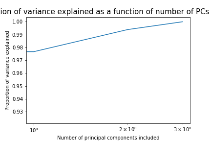
We analyze the PCA for the train set and compare how this would be on the validation set. All of the (useless) features are emitted from all the sets (train, validation, test). In this example we emit the least 2 useful features (The ones that are nessesary to be used in 95% of the cases).
The two emitted features are sepal width and sepal length.
The two remaining features are petal width and petal length.
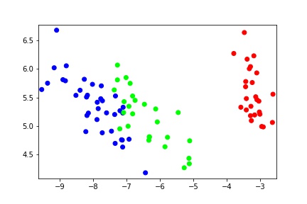
Lets see how the data somewhat looks like in projected 2d plot
Classifiers
We use two classification algorithms to classify after we have emitted the features. The train set is used to find the most optimal parameters for our models.
k- Nearest Neighbours (kNN)
The kNN algorithm works by using nearest points to determine in which group a datapoint should be classified.
For kNN we find the we can achieve a training accuracy of 100% with 3 neighbours.
We do this by running our algorithm kNN for a different number of neightbours. For this algorithm it might be feasible as it is only one parameter that we have to optimize, but for algorithms or models with more parameters it will probably be too computationally inefficient to try it for many parameters. The number of combinations of paramets increase exponentially. Random optimizers such as Adam exists to randomize the choice of parameters and parameter combinations to find the near optimal ones.
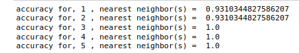
This is the same for higher number of neighbours, but we do not want to make our model too complicated. This would be computationally inefficient, and we risk that we fit our model too much on our training set. So the simpler the solution the better (Ockham’s razor).
Random Forest Classification
N_estimators is number of decision trees in the forest. More trees mean that we will have higher variance and we might overfit our data to the training set. We expect to see a decrease in the error as we are subdividing the set into smaller and smaller classification sets.
n_jobs, computation optimization, should only be related on large datasets due to parralel procession overhead. Starting and switching and combining the data on each core takes time, so the process cannot start immediately. We will choose not to utilize this feature as we have a very small dataset
min_sample_split is the number of branches that are split at the end. So at the bottom of the tree (where the leafes are). We will for each branch have two leafes or less when we set this equal to two.
Random forest usually have the downside of favoring high cardinality features, as we branch into many smaller branches unique, and somewhat niche, features will become increasingly weighted on par with the more general features.
max_depth is how far we go in terms of classifications. If this is set to None we will keep splitting the tree into smaller branches. Eg. if this was set to 3, we would split the initial dataset once and then two times more for each child that we get from the first split.
Predicting on Test set
We then see how our models fare on our test set by predicting with our model. By predicting we mean that we apply the algorithm with the optimized parameters that we found in the training phase.
Lets first start by looking at the kNN classifier.
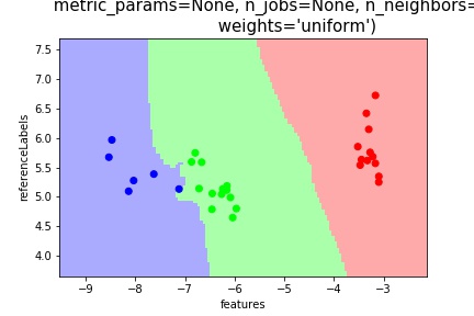
The classifier seems to divide the datapoints fairly clearly into the different labels. There is one datapoint on the border between green and blue that is question, but it still classifies it correctly.
Next lets look at the random forest prediction
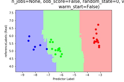
To compare the two classifiers we find that kNN seems more “smooth” as opposed to the randomforest.
Other techniques we could explore in order to better our Randomforest model, could be that we generate multiple random forest and then take the mean of the optimal parameters from these and input them into a final model. This procedure is called Mean Decrease in Impurity (MDI) and can help to smooth out some of the quirkyness that comes with the random forest.