Linear regression - House Prices
- Boston Housing Data - House Price
- TV adds - Sales
- Olympic race data - Time
- Medical Insurance Patients - Cost of Product
This Project aims to visualize some relations between features and their respective values.
In the case of the Boston Housing Data, with different features such as: age of the house, infrastructure in area, ecology, as well as other data about the residents.
To have some indicator of how wrong our predictions are we use the Root Mean Squared Error.
Markdown code
def rmse(t, tp): return numpy.sqrt(numpy.mean(numpy.square(numpy.abs(numpy.subtract(t,tp)))))
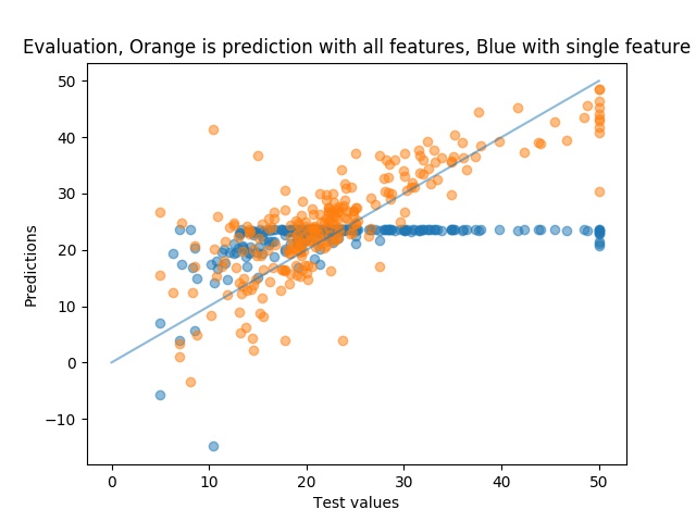
Our error indicators for the first feature and for all the features are as such:
RMSE Single Feature the Column CRIM (per capita crime rate by town): 8.954859906611233
RMSE All features: 6.21287919995914
We can see that when we use all the features we get less error in our predictions.
The plots of the relation between our predictions and our real test values are somewhat better when using all the features. If the predictions and the real values match perfectly they should lie on the straight line.
Cross Validation
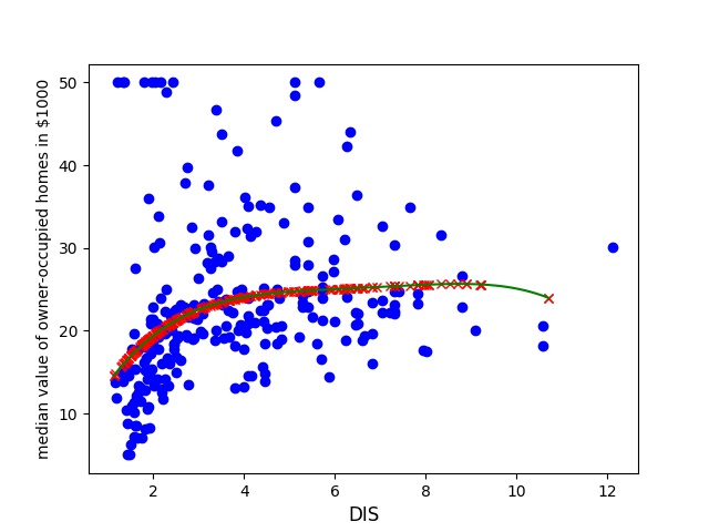
Now lets try to look at each features individually and see if we can find a linear relation between them and the label (our house price).
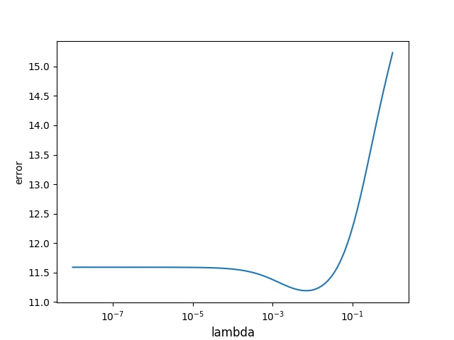
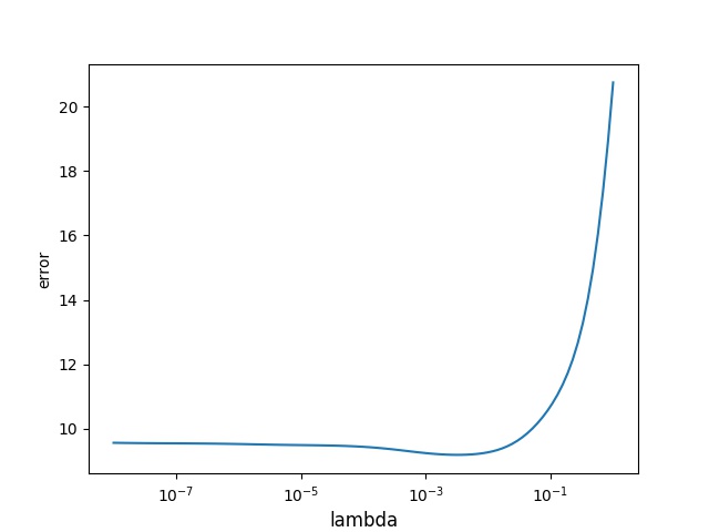
For cross validation we take out 1 datapoint and evaluate and try to predict the 1 datapoint we took out. We do this for a range of lambda values to see which lambda fits the set best.
We individually for each feature explore its impact on the House Price. Some have no linear correlation, while others have a very clear correlation.
For all of the examinations we will use a degree of 4. A degree of 1 means that the data can be explored from two weights (one that influence the feature and one initial, to explain initial conditions at x=0), also indicating that this will be a straight line.
A degree of 4 means that we will have some wiggle room for our classification, while we still dont have a function that is too complicated.
We will start with a weighted value of lambda=0, we will explore different values so that we can minimize the error that we get. Our lambda values range from 10^-8 to 1, we explore 100 values equally distributed in this range.
For example the DIS(weighted distances to five Boston employment centres) feature has a clear linear regression while the
There seems to be a clear linear correlation, and we have a clear trend of convergence towards a housing price of 25 k starting at a Distance of 6 km, although we are still rising. At the end we see a dip, this might be due to lack of data. This is clearly not expected although a possible explanation could be that when we are more than 10 kilometers away we are out of the centrum of the city and housing prices might start to fall off.
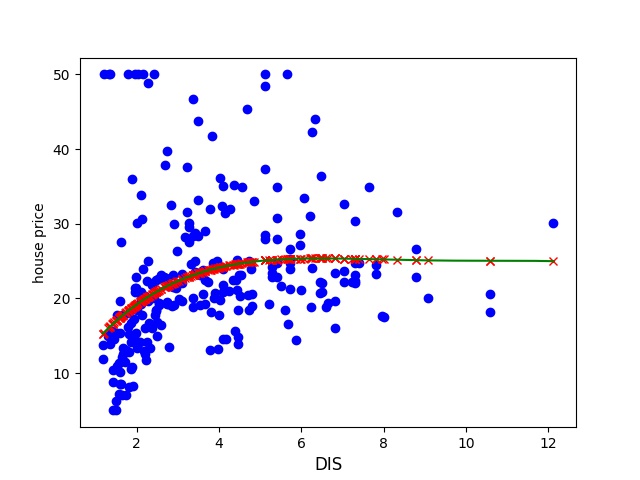
Lets try to do some crossvalidation and see whether we can find a more optimal lambda value.
Lets try to have a look at a different feature, and lets pick one that a negative impact on the housing price.
We find that the NOX (nitric oxides concentration in parts per 10 million) has a clear negative effect, although it seem that if we go up to a concentration of 0.9 it starts it rise again.
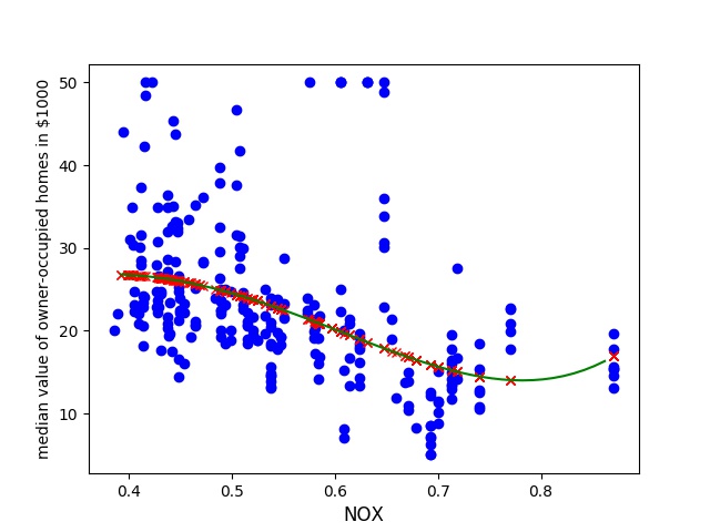
This might be because we overfit to the 3rd or 4th degree. Lets try to optimize the weighted value lambda and see if it favors a lower error on the lower range of nitric oxides values.
Now lets try to see how our prediction looks like now with the updated lambda.
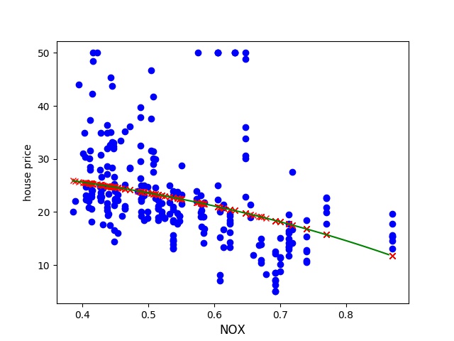
This seems much more feasible. We can see that we have a downwards trend and it is non 1st degree.